4.30.2012

Why visualizing instrumental variables made me less excited about it

Instrumental variables (IV and 2SLS) is a statistical approach commonly used in the empirical social sciences ("instrumental variables" has > 84,000 hits on google scholar) but it often seems to be over-interpreted. I realized this when, as a grad student, I tried to draw a graphical description of what IV was doing. Ever since, I've never bothered to estimate IV and only spend my time on reduced form models.  These are my two cents.

IV & 2SLS

IV was originally developed to combat attenuation bias in ordinary least-squares, but somebody (I don't know who) realized it could be used to estimate local average treatment effects in experimental settings when not all subjects in a treatment group actually received the treatment of interest.  From there, someone figured out that IV could be used in retrospective studies to isolate treatment effects when assignment to treatment had some endogenous component. This last interpretation is where I think a lot of folks run into trouble. (If you don't know what any of this means, you probably won't care about the rest of this post...)

All of these conceptual innovations were big contributions.  But what happened afterwards led to a lot of sloppy thinking.  IV is often taught as a method for "removing" endogeneity from an independent variable (variable X) in a regression.  While strictly a correct statement (if some relatively strong assumptions are met), it often feels as if it's abused.  My perception from papers/talks/discussion is that most students interpret IV in a similar way to how they interpret a band-pass filter: if you find a plausible instrument (variable Z), you can "filter out" the bad (endogenous) part of your independent variable and just retain the good (exogenous) part.  While a useful heuristic for teaching, its overuse leads to bad intuition.

IV with one instrument

The first stage regression in IV "filters out" all variation in X that does not project (for now, linearly) onto Z.  This linear projection is just Z*b, but it is often written as "X-hat". While not mathematically incorrect, and appealing for heuristic purposes, I think that using X-hat as a notational tool is why a lot of students get confused. It makes students think that X-hat is just like X, except without all the bad endogenous parts.  But really, X-hat is more like Z than it is like X. In fact, X-hat IS Z! It's just linearly rescaled by b, which is just a change in units.  The reason why X-hat is exogenous if Z is exogenous is because

X-hat = Z * b

where b is a constant. It seems silly and patronizing to reiterate an equation that is taught in metrics 101 a gazillion times, but people seem to forget that this little rescaling equation is doing all the heavy lifting in an IV model.  (I bet that if we never used "X-hat" notation and we renamed "the first stage" something less exciting, like "linearly converting units," then grad students would think IV is much less magical...)

Once X-hat is estimated, it is used as the new regressor in the "second stage" equation

Y = X-hat * a + error

and then a big fuss is made about how a is the unbiased effect of X on Y.  But if we drop the X-hat notation and replace it with the rescaled-Z notation, we get something less exciting:

Y = Z * b * a + error

Where a is now the unbiased effect of Z on Y, but rescaled by a factor 1/b.  For those familiar with IV, this looks a lot like the reduced form equation

Y = Z * c + error

which was always valid because Z is exogenous. Clearly,

a = c / b.

If you're still reading, you should be yawning, since this all seems very boring: these are all just variations on the same reduced form equation. And that's my main point, which I don't think is taught enough: Instrumental variables is only as good as your reduced form, because it is a linear rescaling of your reduced form. Of course, there are adjustments to standard errors, but if you're doing IV to remove bias, then you were focused on your point estimate to begin with. (An aside: it drives me nuts when people are "uninterested" in the reduced form effect of natural variations [eg. weather] on some outcome, but then are fascinated if you use the same variation as an instrument for some otherwise endogenous intermediate variable. The latter regression is the same as the first, only the coefficient has been rescaled by 1/b!)

Enough ranting. How do we visualize this? Its as easy as it sounds: you rescale the horizontal axis in your reduced form regression.

To illustrate this, I generated 100 false data points with the equations

Z ~ uniform on [0,1]
X =  Z * 2 + e1
Y = X + e2


where e1 and e2 are N(0,1). And then plot the reduced form equation (Z vs. Y) as the blue line in the upper-left panel:


I then estimate the first stage regression in the lower left panel and show the predicted values X-hat as open red circles. In the lower right panel, I just plot X-hat against X-hat to show that I am reflecting these values from the vertical axis (ordinate) to the horizontal axis (abcissa). Then, keeping X-hat on the horizontal axis, I plot Y against X-hat in the upper right panel. This is the second stage estimate from IV, which gives us our unbiased estimate of the coefficient a (the slope of the red line).

[The code to generate these plots in Stata is at the bottom of this post.]

What is different between the scatter on the upper left (blue line, representing the reduced form regression) and the scatter on the upper right (red line, representing the second stage of IV)? Not too much. The vertical axis is the same and the relative locations of the data points are the same. The only change is that the horizontal variable has been rescaled by a factor of two (recall the data generating process above). The IV regression is just a rescaled version of the reduced form.  What happened to X? It was left behind in the lower left panel and it never went anywhere else. It only feels like it is somehow present in the upper right panel because we renamed Z*b the glitzier X-hat.

Multiple instruments (2SLS)

Sometimes people have more than one exogenous variable that influences X (eg. temperature and rainfall). Both of these variables can be used as instruments in the first stage. What happens to the intuition above when we do this? Not too much, except things get harder to draw. But the fact that it's harder to draw doesn't mean that the estimate is necessarily more impressive or magical.

Suppose we have now have instruments Z1 and Z2 such that

Multivariate first stage: X = Z1 - Z2
Second stage: Y = 2 * X

then the first stage regression (X-hat) looks like this:


where the two horizontal axes are Z1 and Z2 and the vertical axis is X.

If we substitute this first stage regression into the second stage, we get

Y = 2 * (Z1 - Z2)

We can easily plot this version of Y as a function of Z1 and Z2 (the reduced form). Here, it's the purple plane:


The resulting second stage regression would take the observed value for Y (purple) and project it onto the predicted values for X (green). The parameter of interest (2 here, but the variable "a" earlier) is just the ratio of the height of the purple surface to the height of the green surface. 

Again, everything can be stated in terms of the instruments Z1 and Z2 (the two horizontal axes), which means the reduced form is again just as good as the second stage.  X only enters by determining how steep the green surface is.

Nonlinear first stage with multiple instruments

Finally, some people use a non-linear first stage.  Again, this is not terribly different. Suppose we have

Nonlinear multivariate first stage: X = Z1^2 - Z2
Second stage: Y = 2 * X

Then the first stage looks like:


and the reduced form regression of Y on Z1 and Z2  is gives us

Y = 2 * (Z1^2 - Z2)

which we overlay in purple again:


Since the second stage didn't change, the height of the purple surface is still always twice the distance from zero relative to the green surface (a scatter plot of pink vs. green values would be a straight line with slope = 2 = a).  This graph looks fancier, but the instruments Z1 and Z2 are still driving everything.  The endogenous variable X only enters passively by determining the height of the green surface. Once that's done, the  Z1 and Z2 do the rest.

Take away: Reduced form models can be very interesting. However, instrumental variables models are rarely much more interesting.  In fact, all the additional interestingness of the IV model arises from the exclusion restriction that is assumed, but this assumption is usually false (recall: how many papers use weather as an instrument?), so the IV model is probably exactly as interesting as the reduced form, except that it has larger standard errors and the wrong units.

[If you disagree, send me a clear visualization of your 2SLS results and all the steps you used to get there.  I'd love to be wrong here.]

4.27.2012

An unusual number of goodies in Nature this week

A special Outlook issue reviewing the challenges of malaria control:

Nature Outlook: Malaria (Open access)
The war against the malaria parasite has raged for millennia, and still claims hundreds of thousands of lives each year. Resistance is a growing issue — for both the parasite to current therapy, and the mosquito to pesticides. Past attempts to eradicate malaria have failed. What will it take to finally subdue this deadly disease?


Commentary on the ivory tower:

Global issues: Make social sciences relevant
Luk Van Langenhove

Excerpt:
The social sciences are flourishing. As of 2005, there were almost half a million professional social scientists from all fields in the world, working both inside and outside academia. According to the World Social Science Report 2010 (ref. 1), the number of social-science students worldwide has swollen by about 11% every year since 2000, up to 22 million in 2006. 
Yet this enormous resource is not contributing enough to today's global challenges, including climate change, security, sustainable development and health. These issues all have root causes in human behaviour: all require behavioural change and social innovations, as well as technological development.... 
Despite these factors, many social scientists seem reluctant to tackle such issues. And in Europe, some are up in arms over a proposal to drop a specific funding category for social-science research and to integrate it within cross-cutting topics of sustainable development. This is a shame — the community should be grasping the opportunity to raise its influence in the real world.... 
Today, the social sciences are largely focused on disciplinary problems and internal scholarly debates, rather than on topics with external impact.... 
The main solution, however, is to change the mindset of the social-science community, and what it considers to be its main goal. If I were a student now, I would throw myself at global challenges and social innovations; I hope to encourage today's young researchers to do the same.


Meta-analysis of a famous question:

Comparing the yields of organic and conventional agriculture
Verena Seufert, Navin Ramankutty & Jonathan A. Foley
Abstract: Numerous reports have emphasized the need for major changes in the global food system: agriculture must meet the twin challenge of feeding a growing population, with rising demand for meat and high-calorie diets, while simultaneously minimizing its global environmental impacts1, 2. Organic farming—a system aimed at producing food with minimal harm to ecosystems, animals or humans—is often proposed as a solution3, 4. However, critics argue that organic agriculture may have lower yields and would therefore need more land to produce the same amount of food as conventional farms, resulting in more widespread deforestation and biodiversity loss, and thus undermining the environmental benefits of organic practices5. Here we use a comprehensive meta-analysis to examine the relative yield performance of organic and conventional farming systems globally. Our analysis of available data shows that, overall, organic yields are typically lower than conventional yields. But these yield differences are highly contextual, depending on system and site characteristics, and range from 5% lower organic yields (rain-fed legumes and perennials on weak-acidic to weak-alkaline soils), 13% lower yields (when best organic practices are used), to 34% lower yields (when the conventional and organic systems are most comparable). Under certain conditions—that is, with good management practices, particular crop types and growing conditions—organic systems can thus nearly match conventional yields, whereas under others it at present cannot. To establish organic agriculture as an important tool in sustainable food production, the factors limiting organic yields need to be more fully understood, alongside assessments of the many social, environmental and economic benefits of organic farming systems.


Copyright Nature


And some interesting agent-based modeling from Nature Climate Change:

Emerging migration flows in a changing climate in dryland Africa
Dominic R. Kniveton, Christopher D. Smith & Richard Black

Fears of the movement of large numbers of people as a result of changes in the environment were first voiced in the 1980s (ref. 1). Nearly thirty years later the numbers likely to migrate as a result of the impacts of climate change are still, at best, guesswork2. Owing to the high prevalence of rainfed agriculture, many livelihoods in sub-Saharan African drylands are particularly vulnerable to changes in climate. One commonly adopted response strategy used by populations to deal with the resulting livelihood stress is migration. Here, we use an agent-based model developed around the theory of planned behaviour to explore how climate and demographic change, defined by the ENSEMBLES project3 and the United Nations Statistics Division of the Department of Economic and Social Affairs4, combine to influence migration within and from Burkina Faso. The emergent migration patterns modelled support framing the nexus of climate change and migration as a complex adaptive system5. Using this conceptual framework, we show that the extent of climate-change-related migration is likely to be highly nonlinear and the extent of this nonlinearity is dependent on population growth; therefore supporting migration policy interventions based on both demographic and climate change adaptation.

4.26.2012

Which number from 2011 is bigger: Apple revenue or global insured losses to all weather disasters?

Answer: Apple revenue.

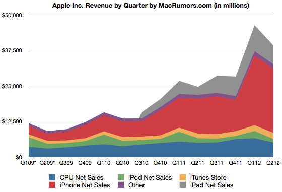
In my line of work, it's good to cultivate a sense of scale for ridiculously large numbers.  So when I saw this on MR:
For the quarter, Apple posted revenue of $39.2 billion and net quarterly profit of $11.6 billion... 

From Macrumors

I thought, "Wow, that's the same order of magnitude as this:"

From Swiss Re Sigma

Except, when integrated across four quarters, Apple is larger (~$100B) than global insured losses to weather (~$60B).

But before you run off thinking that weather isn't costly, remember that only a fraction of all weather losses are insured (probably ~5-15% globally, is my guess, but it's a very hard number to pin down). So global losses to weather are probably substantially larger than Apple's revenue, at least until iPhone 5 is released...

4.25.2012

Background reading on global institutions

Reading about recent cases in the international criminal court, I realized that I don't actually know much about how the court really functions.  So I went looking for a primer on the ICC and found something in the "Global Institutions Series" published by Routledge (and subsequently remembered that I wanted to blog this series a while back).

I discovered this series when I went looking for background reading on how the UNHCR functions.  I found this book by Loescher et al (pictured), which gave a comprehensive background of the institution in a concise 130 pages (useful for us busy folk).  On the inside flap is a list of other volumes that have been assembled, covering institutions from the WHO and the IMF to the International Olympic Committee (see the complete list here).  They seem like an imminently practical resource and I've ordered a few more. I may even end up using some in future classes.  (FE readers might be interested in the volume on global environmental institutions, which I found in a free online PDF here).  The series began in 2005, so some of the volumes might be missing the most recent debates. But for the historical context of these institutions, many of which formed around mid-century (last century), I don't think that should matter much.

This is the publisher's summary of the series:
The "Global Institutions Series" is edited by Thomas G. Weiss (The CUNY Graduate Center, New York, USA) and Rorden Wilkinson (University of Manchester, UK) and designed to provide readers with comprehensive, accessible, and informative guides to the history, structure, and activities of key international organizations as well as books that deal with topics of key importance in contemporary global governance. Every volume stands on its own as a thorough and insightful treatment of a particular topic, but the series as a whole contributes to a coherent and complementary portrait of the phenomenon of global institutions at the dawn of the millennium. 
Books are written by recognized experts, conform to a similar structure, and cover a range of themes and debates common to the series. These areas of shared concern include the general purpose and rationale for organizations, developments over time, membership, structure, decision-making procedures, and key functions. Moreover, current debates are placed in historical perspective alongside informed analysis and critique. Each book also contains an annotated bibliography and guide to electronic information as well as any annexes appropriate to the subject matter at hand.

4.24.2012

Interfacing Water, Climate, And Society: A Resource List

The Research Applications Laboratory at NCAR has a nice wiki-like resource list for folks interested in the interface between water, climate and society. The list isn't comprehensive, but its useful and has sections on:
  • Undergraduate Level Degree Programs
  • Graduate Level Degree Programs
  • Post-graduate Opportunities
  • Academic Research Groups
  • Professional Development and Research Training
  • Professional Networks
  • Boundary Organizaions
  • Journals
  • References
  • Funding Programs
  • Conferences
Check it out here.

4.23.2012

Edu-tainment for misanthropic referees

This is very funny, although your amusement will probably be proportional to the number of papers you've reviewed + 4 * the number of papers you've submitted and gotten rejected because of referees.

[The appendix is actually quite serious and addresses a number of real statistical issues, although several are specialized for neuroimaging.]

Ten ironic rules for non-statistical reviewers
Karl Friston

Abstract: As an expert reviewer, it is sometimes necessary to ensure a paper is rejected. This can sometimes be achieved by highlighting improper statistical practice. This technical note provides guidance on how to critique the statistical analysis of neuroimaging studies to maximise the chance that the paper will be declined. We will review a series of critiques that can be applied universally to any neuroimaging paper and consider responses to potential rebuttals that reviewers might encounter from authors or editors.

Excerpt:
There is a perceived need to reject peer-reviewed papers with the advent of open access publishing and the large number of journals available to authors. Clearly, there may be idiosyncratic reasons to block a paper – to ensure your precedence in the literature, personal rivalry etc. – however, we will assume that there is an imperative to reject papers for the good of the community: handling editors are often happy to receive recommendations to decline a paper. This is because they are placed under pressure to maintain a high rejection rate. This pressure is usually exerted by the editorial board (and publishers) and enforced by circulating quantitative information about their rejection rates (i.e., naming and shaming lenient editors). All journals want to maximise rejection rates, because this increases the quality of submissions, increases their impact factor and underwrites their long-term viability. A reasonably mature journal like Neuroimage would hope to see between 70% and 90% of submissions rejected. Prestige journals usually like to reject over 90% of the papers they receive. As an expert reviewer, it is your role to help editors decline papers whenever possible. In what follows, we will provide 10 simple rules to make this job easier: 
Rule number one: dismiss self doubt Occasionally, when asked to provide an expert opinion on the design or analysis of a neuroimaging study you might feel under qualified. For example, you may not have been trained in probability theory or statistics or – if you have – you may not be familiar with topological inference and related topics such as random field theory. It is important to dismiss any ambivalence about your competence to provide a definitive critique. You have been asked to provide comments as an expert reviewer and, operationally, this is now your role. By definition, what you say is the opinion of the expert reviewer and cannot be challenged – in relation to the paper under consideration, you are the ultimate authority. You should therefore write with authority, in a firm and friendly fashion. 
[My favorite: (emphasis added)]
Rule number two: avoid dispassionate statements A common mistake when providing expert comments is to provide definitive observations that can be falsified. Try to avoid phrases like “I believe” or “it can be shown that”. These statements invite a rebuttal that could reveal your beliefs or statements to be false. It is much safer, and preferable, to use phrases like “I feel” and “I do not trust”. No one can question the veracity of your feelings and convictions. Another useful device is to make your points vicariously; for example, instead of saying “Procedure A is statistically invalid” it is much better to say that “It is commonly accepted that procedure A is statistically invalid”. Although authors may be able to show that procedure A is valid, they will find it more difficult to prove that it is commonly accepted as valid. In short, trying to pre-empt a prolonged exchange with authors by centering the issues on convictions held by yourself or others and try to avoid stating facts. 
Rule number three: submit your comments as late as possible It is advisable to delay submitting your reviewer comments for as long as possible – preferably after the second reminder from the editorial office. This has three advantages. First, it delays the editorial process and creates an air of frustration, which you might be able to exploit later. Second, it creates the impression that you are extremely busy (providing expert reviews for other papers) and indicates that you have given this paper due consideration, after thinking about it carefully for several months. A related policy, that enhances your reputation with editors, is to submit large numbers of papers to their journal but politely decline invitations to review other people's papers. This shows that you are focused on your science and are committed to producing high quality scientific reports, without the distraction of peer-review or other inappropriate demands on your time.
[I am definitely guilty of this last one... it goes on]

My own related grievances here.

h/t Matt

4.19.2012

Does surviving violence make you a better person?

Maybe, though it also seems to impact dynamic decision making. Forthcoming in this month's American Economic Review:
Violent Conflict and Behavior: A Field Experiment in Burundi 
Voors, Maarten J., Eleonora E. M. Nillesen, Philip Verwimp, Erwin H. Bulte, Robert Lensink, and Daan P. Van Soest
Abstract: We use a series of field experiments in rural Burundi to examine the impact of exposure to conflict on social, risk, and time preferences. We find that conflict affects behavior: individuals exposed to violence display more altruistic behavior towards their neighbors, are more risk-seeking, and have higher discount rates. Large adverse shocks can thus alter savings and investments decisions, and potentially have long-run consequences—even if the shocks themselves are temporary.

A prior version of the paper is available here, repec here. Of note is this great opening line: "Civil wars are sometimes referred to as 'development in reverse'..."

That said, there is countervailing evidence...:
National Cultures and Soccer Violence 
Edward Miguel, Sebastián M. Saiegh and Shanker Satyanath
Can some acts of violence be explained by a society’s cultural norms?  Scholars have found it hard to empirically disentangle the effects of cultural norms, legal institutions, and poverty in driving violence. We address this problem by exploiting a natural experiment offered by the presence of thousands of international soccer (football) players in the European professional leagues. We find a strong relationship between the history  of civil conflict in a player’s home country and his propensity to behave violently on the soccer field, as measured by yellow and red cards. This link is robust to region fixed effects, country characteristics (e.g., rule of law, per capita income), player characteristics (e.g., age, field position, quality), outliers, and team fixed effects. Reinforcing our claim that we isolate cultures of violence rather than simple rule-breaking or something else entirely, there is no meaningful correlation between a player’s home country civil war history and performance measures not closely related to violent conduct.


4.18.2012

Columbia's IPWSD 2012 is this Friday

The second Interdisciplinary Ph.D. Workshop in Sustainable Development (previously here) is this coming weekend. The workshop is organized by our Ph.D. program's Sustainable Development Doctoral Society
and showcases current work on sustainability issues by Ph.D. students at institutions around the world. The lineup of student papers looks fantastic this year, so if you're in town Friday or Saturday you may want to swing by. The full schedule is available here.

4.16.2012

Cheap parallel computing for students

I don't like to advertise for companies, but Matlab recently released its 2012 version for students and I know that a lot of students don't realize how much computational bang they can get for their buck.  The parallel computing package for Matlab only costs students $29 and allows them to run parallel code on an unlimited number of cores. (Compare this to Stata, which charges hundreds of dollars per additional core.)  And even more importantly, parallelizing your code is amazingly easy (in the best cases, it may only involve changing your "for" commands to "parfor").  As a PhD student, I think this $29 investment saved me several months on my dissertation (I'm not kidding).

I'm guessing there's a similar free package for R which I don't know about (please comment).

4.07.2012

Evaluating 1981 climate predictions

RealClimate has a great piece evaluating predictions in Hansen's et al.'s 1981 Science article "Climate Impact of Increasing Atmospheric Carbon Dioxide":
To conclude, a projection from 1981 for rising temperatures in a major science journal, at a time that the temperature rise was not yet obvious in the observations, has been found to agree well with the observations since then, underestimating the observed trend by about 30%, and easily beating naive predictions of no-change or a linear continuation of trends. It is also a nice example of a statement based on theory that could be falsified and up to now has withstood the test.
The rest is here. The abstract from the original article is worth noting:
The global temperature rose by 0.20C between the middle 1960's and 1980, yielding a warming of 0.4°C in the past century. This temperature increase is consistent with the calculated greenhouse effect due to measured increases of atmospheric carbon dioxide. Variations of volcanic aerosols and possibly solar luminosity appear to be primary causes of observed fluctuations about the mean trend of increasing temperature. It is shown that the anthropogenic carbon dioxide warming should emerge from the noise level of natural climate variability by the end of the century, and there is a high probability of warming in the 1980's. Potential effects on climate in the 21st century include the creation of drought-prone regions in North America and central Asia as part of a shifting of climatic zones, erosion of the West Antarctic ice sheet with a consequent worldwide rise in sea level, and opening of the fabled Northwest Passage.

4.06.2012

Is the AMO our fault?

From this week's Nature, a paper showing evidence that the Atlantic Multidecadal Oscillation is a result of combined human and volcanic aerosol emission patterns:

Aerosols implicated as a prime driver of twentieth-century North Atlantic climate variability
Ben B. B. Booth, Nick J. Dunstone, Paul R. Halloran, Timothy Andrews & Nicolas Bellouin

Systematic climate shifts have been linked to multidecadal variability in observed sea surface temperatures in the North Atlantic Ocean. These links are extensive, influencing a range of climate processes such as hurricane activity and African Sahel and Amazonian droughts. The variability is distinct from historical global-mean temperature changes and is commonly attributed to natural ocean oscillations. A number of studies have provided evidence that aerosols can influence long-term changes in sea surface temperatures, but climate models have so far failed to reproduce these interactions and the role of aerosols in decadal variability remains unclear. Here we use a state-of-the-art Earth system climate model to show that aerosol emissions and periods of volcanic activity explain 76 per cent of the simulated multidecadal variance in detrended 1860–2005 North Atlantic sea surface temperatures. After 1950, simulated variability is within observational estimates; our estimates for 1910–1940 capture twice the warming of previous generation models but do not explain the entire observed trend. Other processes, such as ocean circulation, may also have contributed to variability in the early twentieth century. Mechanistically, we find that inclusion of aerosol–cloud microphysical effects, which were included in few previous multimodel ensembles, dominates the magnitude (80 per cent) and the spatial pattern of the total surface aerosol forcing in the North Atlantic. Our findings suggest that anthropogenic aerosol emissions influenced a range of societally important historical climate events such as peaks in hurricane activity and Sahel drought. Decadal-scale model predictions of regional Atlantic climate will probably be improved by incorporating aerosol–cloud microphysical interactions and estimates of future concentrations of aerosols, emissions of which are directly addressable by policy actions.

A Nature News & Views article on the paper is available here.

4.05.2012

Temperature and generally antisocial behavior


Not only do people honk horns and hit you with baseball pitches more when it's hot out, but you also get worse customer service...

The effects of temperature on service employees' customer orientation: an experimental approach
Peter Kolba, Christine Gockelb & Lioba Wertha

Abstract: Numerous studies have demonstrated how temperature can affect perceptual, cognitive and psychomotor performance. We extend this research to interpersonal aspects of performance, namely service employees' and salespeople's customer orientation. We combine ergonomics with recent research on social cognition linking physical with interpersonal warmth/coldness. In Experiment 1, a scenario study in the lab, we demonstrate that student participants in rooms with a low temperature showed more customer-oriented behaviour and gave higher customer discounts than participants in rooms with a high temperature – even in zones of thermal comfort. In Experiment 2, we show the existence of alternative possibilities to evoke positive temperature effects on customer orientation in a sample of 126 service and sales employees using a semantic priming procedure. Overall, our results confirm the existence of temperature effects on customer orientation. Furthermore, important implications for services, retail and other settings of interpersonal interactions are discussed.

4.04.2012

US Wind Fields Visualization

Following last week's ocean currents animation one of our readers sends us Fernanda Viégas and Martin Wattenberg's real time Wind Map:

The wind map is a personal art project, not associated with any company. We've done our best to make this as accurate as possible, but can't make any guarantees about the correctness of the data or our software. Please do not use the map or its data to fly a plane, sail a boat, or fight wildfires...
Surface wind data comes from the National Digital Forecast Database. These are near-term forecasts, revised once per hour. So what you're seeing is a living portrait. (See the NDFD site for precise details; our timestamp shows time of download.) And for those of you chasing top wind speed, note that maximum speed may occur over lakes or just offshore. 
We'd be interested in displaying data for other areas; if you know of a source of detailed live wind data for other regions, or the entire globe, please let us know

4.03.2012

The effect of life expectancy on human capital investments


Limited Life Expectancy, Human Capital and Health Investments: Evidence from Huntington Disease
Emily Oster, Ira Shoulson, E. Ray Dorsey

Abstract: One of the most basic predictions of human capital theory is that life expectancy should impact human capital investment.  Limited exogenous variation in life expectancy makes this difficult to test, especially in the contexts most relevant to the macroeconomic applications.  We estimate the relationship between life expectancy and human capital investments using genetic variation in life expectancy driven by Huntington disease (HD), an inherited degenerative neurological disorder with large impacts on mortality. We compare investment levels for individuals who have ex ante identical risks of HD but learn (through early symptom development or genetic testing) that they do or do not carry the genetic mutation which causes the disease.  We find strong qualitative support: individuals with more limited life expectancy complete less education and less job training.  We estimate the elasticity of demand for college completion with respect to years of life expectancy of 0.40. This figure implies that differences in life expectancy explain about 10% of cross-country  differences in college enrollment.  Finally, we use smoking and cancer screening data to test the corollary that health capital is responsive to life expectancy.


4.02.2012

What happens when we relax credit constraints?


Challenges in Banking the Rural Poor: Evidence from Kenya's Western Province
Pascaline Dupas, Sarah Green, Anthony Keats, and Jonathan Robinson

Most people in rural Africa do not have bank accounts. In this paper, we combine experimental and survey evidence from Western Kenya to document some of the supply and demand factors behind such low levels of financial inclusion. Our experiment had two parts. In the first part, we waived the
fixed cost of opening a basic savings account at a local bank for a random subset of individuals who were initially unbanked. While 63% of people opened an account, only 18% actively used it. Survey evidence suggests that the main reasons people did not begin saving in their bank accounts are that: (1) they do not trust the bank, (2) service is unreliable, and (3) withdrawal fees are prohibitively expensive. In the second part of the experiment, we provided information on local credit options and lowered the eligibility requirements for an initial small loan. Within the following 6 months, only 3% of people initiated the loan application process. Survey evidence suggests that people do not borrow because they do not want to risk losing their collateral. These results suggest that, while simply expanding access to banking services (for instance by lowering account opening fees) will benefit a minority, broader success may be unobtainable unless the quality of services is simultaneously improved. There are also challenges on the demand side, however. More work needs to be done to understand what savings and credit products are best suited for the majority of rural households.

Click to enlarge